How to Represent Data

DOWNLOADS

Salt Level data sets

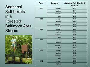
Seasonal – Forest Area

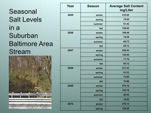
Seasonal – Suburban Area

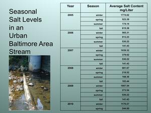
Seasonal – Urban Area

Annual – Combined Areas

How to Represent Data slide show

How to Represent Data teacher's guide

TEACHER'S GUIDE

Begin slideshow.  Slides 1-5 discuss how population density impacts salt levels.

Discussion

Key Idea: Salt will be most abundant in areas that have many roads and high traffic levels due to differences in population densities.

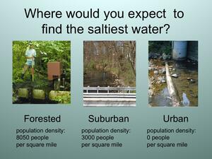
Question:  Where do you expect to find the saltiest water - urban, suburban or forested locations?
Answer:  In an urban location because there are more roads

Question:  Where do you expect to find the least salty water - urban, suburban or forested locations?
Answer:  In a forested areas because there aren’t any roads

Question:  How would you test these predictions? Look back at your data.  What type of data are we using?
Answer:  Seasonal and location data, therefore, we would need to analyze data from forested, suburban, urban locations to see whether water in urban locations is saltier and whether salt levels increase in the winter.

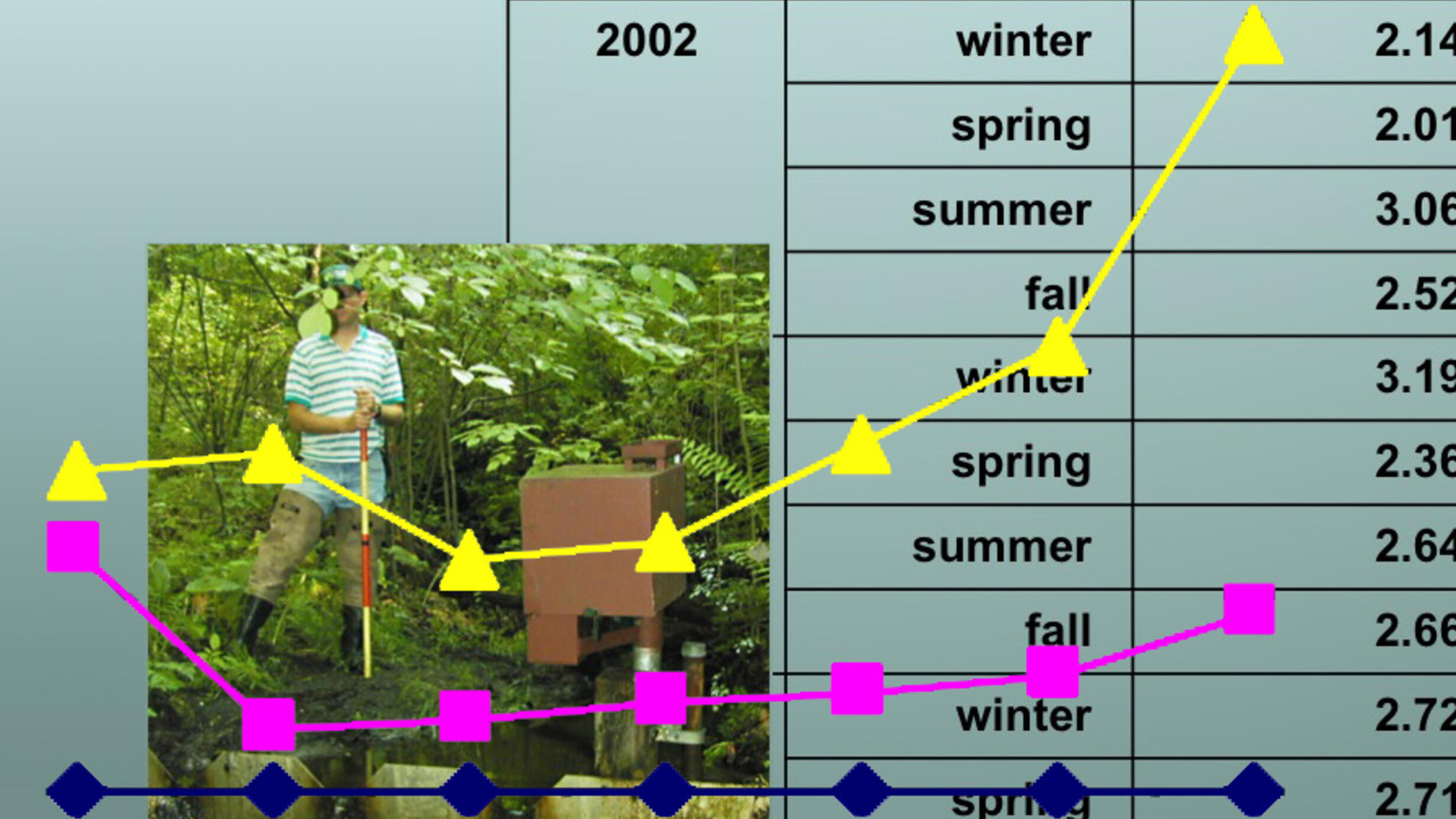
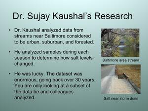
Slide 6 summarizes the data and research the students are analyzing. It says:

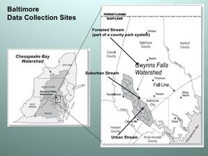
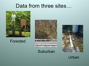
• Dr. Kaushal analyzed data from streams near Baltimore considered to be urban, suburban, and forested.
• He analyzed samples during each season to determine how salt levels changed.
• He was lucky. The dataset was enormous, going back over 30 years. You are only looking at a subset of the data he and his colleagues analyzed.

Key Idea: The annual salt levels might differ in forested, suburban, and urban streams (because of roads).

Each area has a different population density that directly reflects how many roads are near the study streams - the greater the density of people, the greater the number of roads.

• Forest: Although people walk and drive to the forest, no people live in it.
• Suburban stream: population density ~3000 people/mile²
• Urban stream population density ~8000 people/mile²

Note for perspective: The population density of New York City is 26,403 people/mile^2, more than any other city in the U.S.  The next highest population density is San Francisco with 17,323 people/mile².

Discussion

Give students time to examine the datasets to determine how to best represent the data. This examination will lead to a discussion of how best to represent the data for analysis. The slideshow also contains slides of the datasets, so the class can more easily discuss them as a group.

Key Idea:  Scientists carefully choose ways to represent data based on needs for analysis.

Question:  Data tables are a form of raw data, which must be analyzed by scientists to draw conclusions.  What is the best way to represent the data so that the different datasets can be easily compared? 
Answer:  A graph, because graphs make it easy to look at patterns in data.

Question:  When creating a graph, what data goes on the x-axis? What data goes on the y-axis? Look at the columns in your data tables to see what type of data you have.
Answer: 

• x-axis: Time (years, seasons) (independent variable)
• y-axis: Salt levels (dependent variable)

Note: This would be a good time to introduce the concept of dependent/independent variables, but it is not necessary for the completion of the unit.

Discussion

Key Idea:  The importance of the proper scale on a graph?

Question:  How do you create an appropriate scale for the dataset?
Answer:  (Use the sample graphs of growth of money over time—Maya and John’s investment income—in the slideshow.)

Discussion

Key Idea: Scientists must choose the right scale for a graph so the data can be correctly analyzed.

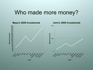
Slide 11:  The two graphs show Maya and John’s investment income from 2009. The graphs show the same growth in income, but are different scales, which make it look like Maya made more money than John. (Teachers Note: They both earned the same income)

Question:  Who made more money, Maya or John?
Answer:  Most students will answer Maya because of the differences in scale, however they both made the same amount. 

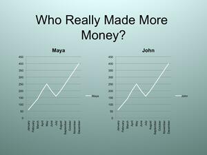
Slide 12: The next slide which shows both investments on the same scale.
Question:  Who really made more money?
Answer:  Both Maya and John made the same amount of money.

Question:  How is it possible for both of them to be making the same income with this graph, but for it to appear as if Maya is making more money on the previous graph if both graphs are of the SAME data?
Answer:  The scale was different on both graphs, which made it look like Maya had a bigger increase, even though her total investment income was the same as John’s.

Question:  Why is it important to choose an appropriate scale for your data?
Answer:  If the scales are different, you cannot compare the data.

Question:  Examine your datasets from forested to suburban, and decide what scale you would like to use for your graphs. What should be the biggest number on the Y axis? Remember you need to take into account the forested, suburban, and URBAN data.
Answer:  Come to a conclusion as a class, each student MUST have the same scale, so that the graphs can be compared. 

Note:  Numbers vary from as low as 2 mg/L of salt for forested areas and as high as 1800 mg/L for urban areas. However,ALLgraphs, even the forested area, must use the same scale that reaches 1800 mg/L.  A labeled graphing template is included in the materials for this lesson.