Overview
Part of the River Ecology Curriculum Collection.
 © AMNH
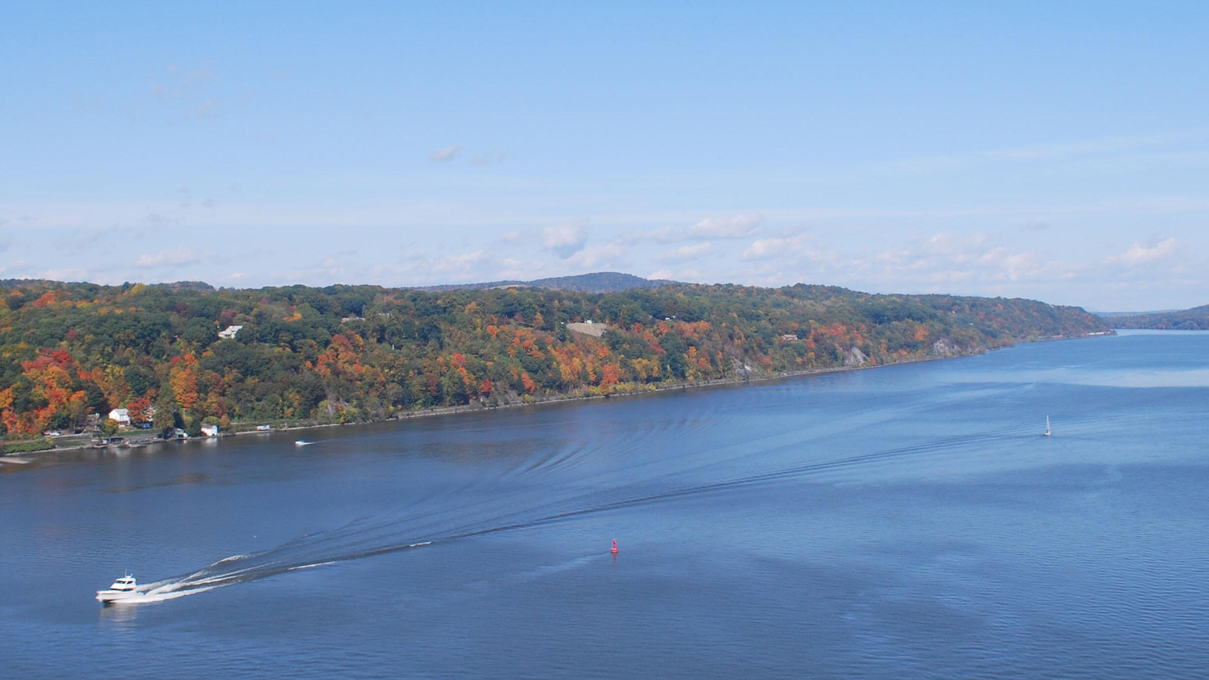
Long before Englishman Henry Hudson explored it in 1609, this majestic river was well traveled by Native Americans. Located in New York State, the Hudson was America's most celebrated and commercially important waterway for 200 years, until the Mississippi Valley was settled. Its beauty has inspired countless writers and artists, including the painters of a movement called the "Hudson River School." The Hudson River flows south about 500 kilometers (km) (310 miles) from the Adirondack Mountains to New York Harbor.
The tidal freshwater portion of the river extends about 163 km (100 miles) from the Troy Dam just north of Albany to Haverstraw Bay, not far from New York City.
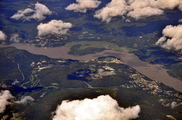
The difference between high and low tide can be as much as 1. 6 m (5.2 feet), and when the tide floods in from the Atlantic Ocean it actually causes the river to reverse direction and flow North! Much of its currents do not come from downhill flow but from these twice-daily tides. As a result, water makes its way down the river quite slowly, taking about 126 days to travel from Troy to the Battery in New York City.
With an average depth of 9.4 meters (31 feet), the water is high in nutrients, fairly turbulent (or well-mixed) because of the tides, and quite cloudy (containing a lot of sediment) from all the mixing.
The lower portion of the Hudson River extends from just south of Newburgh, NY to the southern tip of Manhattan. It is an estuary, where salty seawater mixes with fresh. Some organisms, like the zebra mussel, can't survive in salty or brackish water. They live only in the upper, freshwater portion of the river, which is the focus of this site.
The Zebra Mussel Invasion
Zebra mussels were first spotted in the Hudson River in May 1991, and probably introduced unintentionally. The larvae are only visible through a microscope and can travel in very small amounts of water. The adults can "hitchhike" on marine equipment like boat trailers and outboard motors, and spread when they spawn in the new water body. Zebra mussels had invaded the Great Lakes in 1988 (probably traveling from Europe in the ballast water carried by ships), and Cary scientists reasoned that a Hudson River invasion was likely. Within 16 months of their introduction, the mussels had spread throughout the freshwater tidal Hudson ecosystem.
Scientists at the Cary Institute of Ecosystem Studies in Millbrook, NY, have been monitoring the Hudson's tidal freshwater ecosystem since 1986, several years before zebra mussels appeared. That was fortunate, because it's rare to have data about a river or lake from before and after an invasion. In this case, scientists have been able to document the effects on the river's ecosystem by comparing their unique before-and-after datasets.
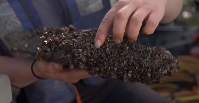
Zebra mussels can live for four to five years, and can grow to about 4 cm (1.57 inches) in length. Females can lay over one million eggs in a spawning season, and populations can reach astonishing levels of 10,000 mussels per square meter — or higher. They attach themselves firmly to hard surfaces on the riverbed with thread-like strands called byssal threads, which makes them hard to dislodge. They also attach to pipes, the bottoms of boats, and even to native mussels, which cannot then survive.
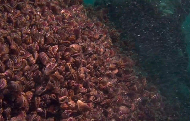 Zebra mussel populations can reach astonishing levels of 10,000 mussels per square meter — or higher.
© AMNH
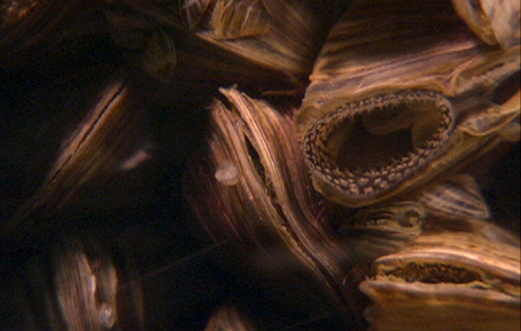 Zebra mussels pump water through their gills to filter out particles of food (primarily phytoplankton).
© AMNH
Zebra mussels are filter feeders: they pump water through their gills to filter out particles of food (primarily phytoplankton). A large population of zebra mussels can filter a volume of water equal to all of the water in the Hudson River estuary every 1-4 days, removing so much plankton and particles that they upset existing food webs. The zebra mussel invasion caused large changes in the fish community of the tidal freshwater Hudson, the near extinction of native pearly mussels, and additional changes to the river's physical and biological characteristics.
Humans are also affected. Zebra mussels clog water pipes, and power plants and businesses that use river or lake water have had to spend millions of dollars on removing them. The mussels can also damage engines, docks, and equipment, and their shells wash up in large numbers on beaches.
Ecosystems are highly complex, however, and can respond to an invasive species in unexpected ways. Although zebra mussels have few natural predators in North America, populations in the Hudson have declined somewhat in recent years. Scientists are working to figure out why. Can you help them? Can you find other ways in which the river has changed since 1992, when the zebra mussel arrived?
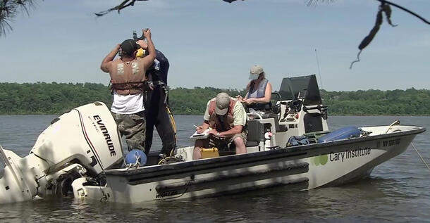
Observing the River
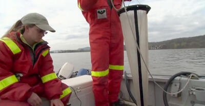
The data you'll be using has been collected by Cary Institute scientists, who've been sampling the tidal freshwater portion of the Hudson River at specific stations for many years. Launching a small motorboat called a Boston Whaler from various points along the river, they systematically draw water samples at precise locations repeatedly over time.
The scientists collect samples according to two different plans:
Transects
This approach consists of collecting water samples at closely-spaced intervals (every 2-4 km (1.2-2.5 miles)) along a 170 km (105 miles) stretch of the river over 1-3 days. Scientists launch a boat at the northern end of the river and sample in the main channel while traveling downriver, usually between Castleton and Haverstraw Bay.
Cardinal stations
These six key stations — Castleton, Hudson, Kingston, Poughkeepsie, Fort Montgomery and Haverstraw Bay — are spread along some 150 km (93 miles) of the tidal freshwater Hudson River. The scientists measure the concentrations of more characteristics at the Cardinal stations than they do during the transects, but cannot sample them all on the same day. These include oxygen, nutrients like nitrogen and phosphorus, and different types of plankton like rotifers. This makes it possible to compare many variables across time.
The scientists then test the samples for a number of factors:
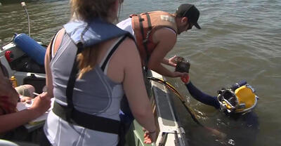
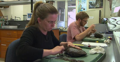
Zebra mussels
Twice in the summer scuba divers collect ten rocks from the hard or rocky areas of the river bottom from each of the seven sampling sites. They bring these rocks back to the lab in, count the number of mussels attached to each, and measure shell length. Samples are archived in ethyl alcohol and stored in the freezer. In “soft-bottom” areas, scientists use a device called a benthic grab to collect material at 48 random sites throughout the freshwater portion of the river. Back in the lab, the material is sieved, and all bivalves counted and identified. A subset is measured for shell length. Since scientists knew approximately how much of the river bottom is rocky and how much is soft, they combine these averages for an annual estimate of the total number of mussels in the freshwater portion of the river, as well as the average per unit of river bottom.
Total Suspended Solids (TSS)
Researchers determine the amount of Total Suspended Solids (TSS) in the river water by pouring a precise amount through a pre-weighed filter. Material too large to pass through is considered “particulate” (a suspended solid), while the material that passes through the filter is considered “dissolved”. After the filter dries, it’s weighed again. The difference is a dry weight measure of the particulates in the water sample. TSS is measured in milligrams per litre (mg/l).
Chlorophyll
Chlorophyll correlates with the amount of phytoplankton in the river. To measure it, researchers pass water samples through filters. The chlorophyll is extracted from the particles that collect on the filters and measured with a device called a fluorometer, which measures the fluorescence of chlorophyll.
Temperature and Dissolved Oxygen
Researchers lower probes into the river that measure temperature, dissolved oxygen, as well as other variables such as pH and conductivity.
Zooplankton (bacteria, copepods, rotifers, cladocera)
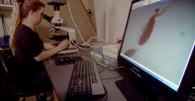
Small zooplankton (micro-zooplankton) are sampled by passing two liters of river water through a fine mesh net. Large zooplankton (macro-zooplankton) are sampled by pumping 100 liters of river water through a net with a larger mesh. The samples are preserved in formaldehyde aboard the boat, carried to the lab, and counted using different microscopes. The microscope depends on the size of the specimens and the volume of the sample.

Shaping Ecosystems
Biotic aspects
Biotic means "living." The biotic components of an ecosystem are the living organisms that inhabit it. These components could include producer organisms, consumer organisms, and decomposers. The key biotic components of the zebra mussel's environment include algae (chlorophyll), bacteria and small zooplankton (which the mussels may consume), and predators such as fish, crabs and birds.
Let's take a closer look at two of these biotic factors: zebra mussels and phytoplankton.
Zebra mussels
This graph shows the number of zebra mussels occupying the bottom of the Hudson River, in units of numbers of mussels per square meter (zm/m2). Zebra mussels thrive on a hard surface or substrate like underwater rocks, and do less well on soft surfaces or substrates like muddy bottoms.
Each year, scuba divers in the Hudson River randomly pick rocks from the hard or rocky areas of the river bottom. They count the number of mussels attached to the rocks, and measure their shell sizes. Scientists use a device called a benthic grab to look for zebra mussels in "soft-bottom" areas, and they count the mussels they find in these samples too.
Since scientists know approximately how much of the river bottom is rocky and how much is soft, they can combine these averages for an annual estimate of the total number of mussels in the freshwater portion of the river, as well as the average per unit of river bottom.
This graph shows that substantial numbers of zebra mussels were first observed in the Hudson River in 1992. At that time the average population size was 4,000 per square meter of river bottom. We can see that since then the numbers have changed each year, from a high of 4,000 mussels/m2 to a low of about 500 mussels/m2 in 2003… (step the viewer through the sample graph)
Phytoplankton
In the Hudson River, the predominant producer organisms are phytoplankton and rooted aquatic macrophytes (large, plant-like structures that grow from the river bottom in shallow areas). Phytoplankton are microscopic organisms that carry out photosynthesis while floating or drifting in the water column. Many consumer organisms eat phytoplankton, making them an important part of the food chain.
Chlorophyll gives many types of producer organisms — which include plants, algae and some types of bacteria — their green color. Chlorophyll is vital for photosynthesis, the process by which producers convert sunlight to energy. It is an indicator of the abundance of these producer organisms.
Chlorophyll concentration is used to measure phytoplankton abundance because it's produced by phytoplankton and is easy to measure. In order to determine the amount of phytoplankton in a water sample, scientists filter out the plankton particles and extract and measure the amount of chlorophyll they contain.
This example shows that chlorophyll in the Hudson River varies between 44.28 mg/L and 0.27mg/L. Concentrations are highest in the summer, when daylight is most abundant and temperatures are highest.
Abiotic aspects
Abiotic means "non-living." The abiotic aspects of an ecosystem are its non-living chemical and physical characteristics. These factors affect the kinds of organisms that can inhabit a given ecosystem, and their abundance. Abiotic factors in an aquatic environment like the Hudson River include the temperature of the water, how much oxygen it contains, how acid or basic it is (pH), how fast or slowly it moves, and how much sunlight penetrates the surface. Additional factors include how much suspended sediment the water contains and its nutrient concentrations (nitrogen and phosphorus).
Let's take a closer look at a few of these abiotic factors.
Temperature
this affects the metabolic rate of organisms. (Metabolism is the set of chemical reactions within organisms that keeps them alive, such as digestion. Their metabolic rate affects their health and growth.) Temperatures fluctuate in the short term as weather changes, over the longer term as seasons change, and over even longer periods as climate changes. The life cycle stages of many organisms change with the season, as do air and water temperatures and the number of hours of daylight.
In this example, which measures temperature in Celsius… (step the viewer through the sample graph)
Dissolved oxygen
Organisms in aquatic environments must adapt to lower concentrations of oxygen than organisms directly exposed to air. This is because O2 must be dissolved in the water to reach them, and water holds nowhere near as much oxygen as does air in Earth's atmosphere. (We're talking here about the kind of oxygen that organisms, including humans, are able to breathe (diatomic oxygen gas, or O2). The oxygen atoms in the water molecule (H2O) are not available for respiration.)
Dissolved oxygen gas (DO) is measured in milligrams O2 per liter (mg/L), which is equivalent to parts per million (ppm), a unit of measurement commonly used when the relative value is very small. At 20°C, river water saturated with O2 holds 9.1 mg/L (or 9.1 ppm) — only 0.00091% of water by weight. By contrast, the atmosphere is 20.9% oxygen!
When oxygen in water is in equilibrium with the atmosphere at a specific temperature, we say it is 100% saturated. The colder the water, the more oxygen can dissolve in it before it reaches saturation. If the water we described above were to be cooled to 10°C, it could hold up to 11.3 mg/L O2 — 25% more oxygen than at 20°C. If the dissolved oxygen concentration of water is below 2 mg/L (or ppm), conditions are "hypoxic" and can stress aquatic organisms.
A number of factors affect the amount of dissolved oxygen in aquatic environments. Producers release O2 during photosynthesis, which can cause oxygen concentrations to be higher in the day than at night. Consumers take up oxygen during respiration, which also influences concentrations. So can temperature fluctuations.
Suspended solids
Total suspended solids (TSS) refers to the solid particles that are suspended in water, which is an important indicator of water quality. TSS is measured by pouring a water sample through a pre-weighed filter. Material too large to pass through is considered "particulate" (or a suspended solid), while the material that passes through the filter is considered "dissolved." The amount of suspended solids is determined by drying and weighing the filter that contains the trapped particles.
TSS may be composed of both biotic particles (such as phytoplankton) and abiotic particles (such as silt and clay). TSS is important to aquatic producer organisms because suspended particles scatter and absorb sunlight, which affects the amount of light available for photosynthesis. TSS also affects many consumer organisms because some portion may be edible. Also, if there's too much particulate matter in the water, it can harm the many aquatic organisms that filter feed, such as mussels and other bivalves.
Introduction to Graphing Data
Changes along the River
Many of the Hudson River's characteristics change along its course. For example, tributaries (streams or smaller rivers that flow into the main portion of the river) increase the volume of the upper (northern) portion of the river, while the lower portion is also an estuary, where freshwater mixes with saltwater from the Atlantic Ocean. Characteristics that change include the river's depth, width, rate of flow, biological communities, and type of bottom (rocky versus soft).
Because these characteristics affect biotic and abiotic variables, it can be helpful to view data collected at one time but across multiple locations. Comparing these variables across space, rather than time, can reveal certain patterns.
Stations along the Hudson River are identified by their distance from the southern tip of Manhattan, which is given a value of RKM 0 (RKM = "river kilometer"). Locations upriver have values that go up, reaching 248 RKM at the Troy Dam north of Albany, New York.
Changes over time
The river also changes over time. The data you're working with was collected over about 20 years. Instead of focusing on geography, you might choose to consider how the variable(s) you're interested in change as time goes by. If you keep other factors (such as location) constant, you might attribute patterns you see to the passage of time, or variables associated with the passage of time. For example, if you look at a scale of months, you might see seasonal changes. A scale of years could reflect factors such as the introduction of an invasive species like the zebra mussel, and a scale of decades might reflect factors such as long-term changes in the climate.
The Hudson River experiences four distinct seasons. As the months go by, air and water temperature and hours of daylight all change, as do the stages in the life cycles of many organisms. During the longer days of summer, for example, more light is available to producer organisms and temperatures are higher, so more photosynthesis takes place. Food is more abundant during the summer months as well, so consumer populations tend to grow.
Multiple variables
When you're looking at a graph that displays more than one type of data at a time, you may observe patterns that suggest connections between types of data. This can lead to new questions and ideas to investigate.
This example displays the density of zebra mussels in the Hudson River during the past 20 years. The second variable shows the concentration of chlorophyll (a measure of phytoplankton abundance) at the Kingston, NY sampling station over the same period. The graph shows that zebra mussels first became abundant in the Hudson River in 1992. Beginning that same year, there are no more summer spikes in chlorophyll. This suggests that these two variables might be connected. This may mean that zebra mussels, which feed by filtering suspended particles, are eating the phytoplankton.
Introduction to Analyzing Data
Scatter plot graphs
It can be easy to see how one variable changes across space (location) or time. But sometimes the data contain additional relationships. A scatterplot graph can show visually how these additional relationships are connected to the patterns observed in space or time. Scatterplots show whether a relationship between two variables exists, the strength of that relationship, and its direction. They can also show any outliers (data points that don't fit the pattern).
A scatter plot is produced by plotting two variables on an X-Y graph. The independent variable is represented on the X-axis. This is the variable that is presumed to be causing a change. The dependent variable is represented on the Y-axis. This is the variable that is changing as a result of the independent variable. The resulting correlations may be positive (rising), negative (falling), or neither (uncorrelated). If the pattern of dots slopes from lower left to upper right, it indicates a positive correlation between the variables. (An increase in the X value corresponds to an increase in the Y value.) If the pattern slopes from upper left to lower right, it indicates a negative correlation. (An increase in the X value corresponds to a decrease in the Y value.)
You can draw a line of best fit (called a 'trendline') that shows the correlation between the variables. You can then express this relationship in the form of an equation, which is a mathematical model of how the variables are related. The equation can help you estimate values on the X axis for which there are no actual data.
Let's look at two variables that might be related: density of zebra mussels and chlorophyll concentration? Our independent variable (to be graphed along the X-axis) should be the ecosystem component that we think is causing the change. In this case its density of zebra mussels. Our dependent variable (on the Y-axis) is the component that we think is being affected by the independent variable. In this case, the dependent variable is chlorophyll a. The scatterplot shows a negative correlation since the trendline is sloping down. This shows that when the density of zebra mussels increases, chlorophyll a decreases.